State Transitions of Distributed Systems

This page describes timelines that represent executions of a distributed system, dataflow graph abstractions of timelines, and states and state transitions of distributed systems.

Timelines

The diagram below shows the timeline of the execution of a distributed system with agents X, Y, Z. The horizontal axis represents time flowing from left to right. Each horizontal line represents the state of one agent. For example, the top horizontal line represents the state of agent X at different points in time, the middle line shows the state of agent Y over time, and the lowest line shows states of Z at all points in time.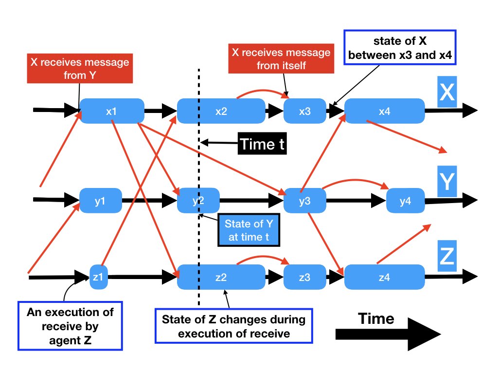

The blue boxes represent executions of receive functions. The red lines represent messages. A message to an agent is from another agent or from itself. Each receive function receives and processes exactly one message. So, each blue box has exactly one input red line.

Each receive is labeled in the diagram. For example, the sequence of receives for agent X are x1, x2, x3, x4. A message sent by agent Z while it is executing receive z1 is received by agent X which causes X to execute receive X2.

The state of an agent between successive receives is represented by the label (not shown) of the edge between the receives. For example, the state of agent X between receive x3 and x4 is the label of the edge after the end of x3 and before the start of x4.

The initial states of agents and channels are shown by dangling edges which have an end point but no start point. For example, initially there is a message that is received by agent X in receive x1 and this message is sent by agent Y. This message is shown by a dangling edge. Similarly there are dangling edges with start points but no end points to depict the final states of agents and channels in this execution. The execution may continue but we are showing only part of it.

The duration of time that an agent takes to execute a receive varies. When an agent executes a statement it may change the agent's variables and change the agent's program counter. So, an agent executes a receive the agent's state changes. The state of an agent at time t is represented in the diagram by the vertical line representing time t.

The state of the system consists of a tuple with an element of the tuple for the state of each component of the system. The components of the system are agents and channels. The state of a channel is a queue representing the sequence of messages in transit along the channel.

The state of the distributed system at time t is depicted by the states of the agents and channels intersected by the vertical line at time t. For example, the state of agent Y at time t is shown in the diagram as the point where the vertical line representing time t intersects the horizontal line representing the timeline of agent Y.

The state of a channel is shown in the diagram by the message lines intersected by the vertical line at time t. For example, there is a message from agent X to agent Y at time t.

Two important points to remember: (1) Message durations are positive and finite but arbitrary. (2) Agent clocks may drift by arbitrary amounts. We don't know how long it takes for a message to get to its destination. We do know that a message will get to its destination eventually, and messages aren't received instantaneously.

An agent can timestamp a message with the time that the agent sends the message where the timestamp is determined by the agent's own clock. But that doesn't tell the receiver of the message when the message was sent as measured by the receiver's clock.

Later, we will look at systems that don't make the assumptions that message durations are unbounded or that agent clocks drift by arbitrary amounts. For the time being, we will see the important consequences of these two assumptions.

Agent Logs

Suppose each agent keeps a log of its state over time, as measured by the agent's clock. If each agent's clock is perfect then the agent's log is represented by the horizontal line of the agent in the timeline diagram. The next figures shows the logs of agents X, Y and Z

The top diagram of the figure shows the log of agent X, the middle diagram is the log of Y, and the lower diagram is the log of Z.

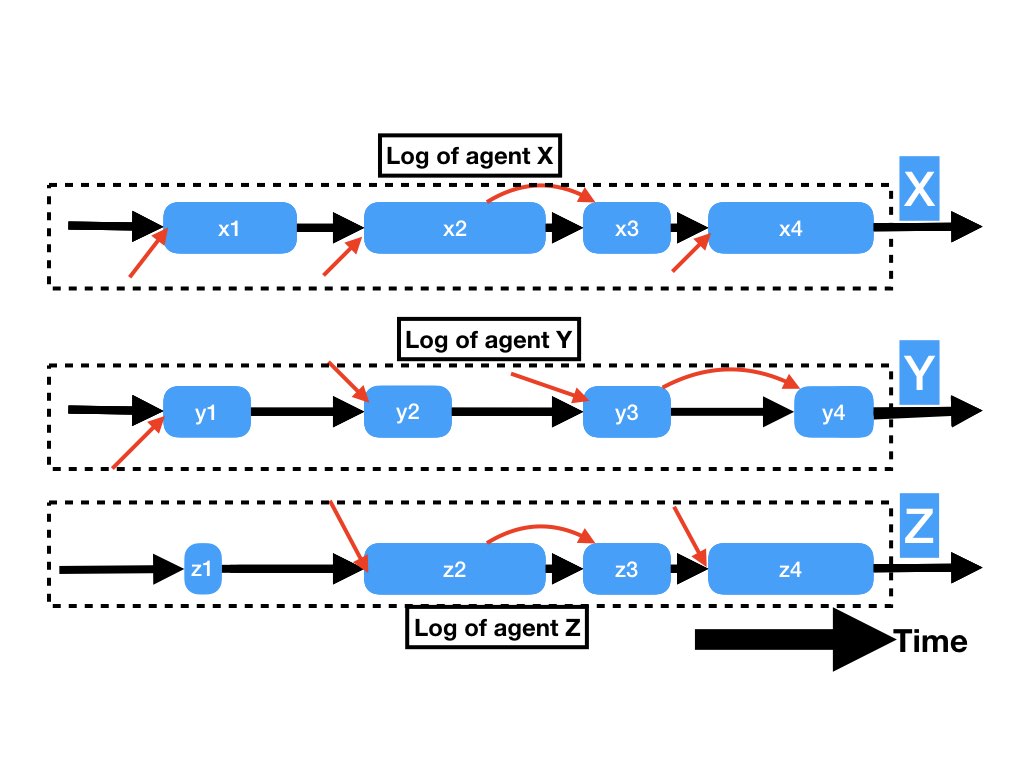
Now suppose the agents send their logs to another agent which puts the agent logs back together to obtain the timeline for the entire system. Can you get the timeline that generated the logs from the logs?

There are several problems. The duration of time for each receive as measured by the agent's clock may not be the true duration. So, we don't know how long each of those blue boxes really is. Okay, then let's simplify the problem assuming that duration of the execution of all receives are the same.

Can we determine the order of receives executed by different agents? Given the logs of figure 2, can you determine whether executions y2 and z2 of receive functions in figure 1 started at the same time, or did y2 start before z2, or z2 before y2? We don't know how long a message takes to get to its destination. So, it's possible that the message received in y2 has a short delay compared to the message received in z2, and so y2 may start before z2. It's also possible that the message delay for the message received in z2 takes less time than the one to y2. So, z2 may start before y2.

In the following diagram agents A and B have the same logs.

In the diagram agent A executes two receives shown as vertices a0 and a1, and agent B executes two receives shown as vertices b0 and b1. Do the agent logs tell us if the receive a1 occurred before the receive b1, or at the same time, or afterwards?

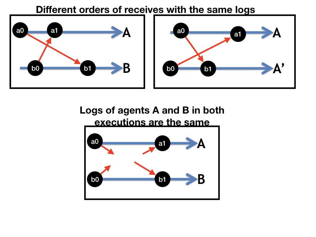
The agent logs don't tell us. We do know that the receive b0 occurred before the receive a1 because a1 receives a message sent during the execution of a1. However, we don't know the relative ordering of a1 and b1.

In figure 1, do we know that z1 occurred before y4?

It's possible that y4 occurs before z1. Here is a possible sequence of executions of receives: x1, y1, x2, x3, y2, y3, y4, x4, z1, z2, z3, z4. But it's also possible that z1 occurs before y4.

Dataflow Graphs

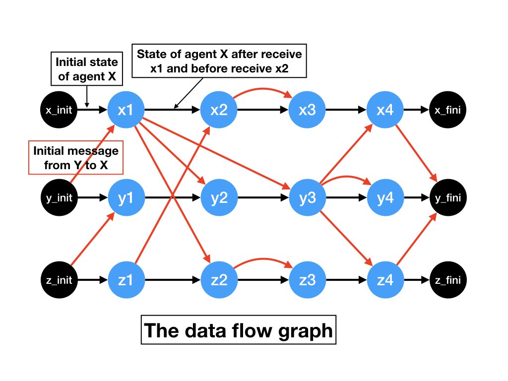
So, what can we get about the execution of the entire system from the collection of agent logs? We can get the dataflow graph which shows the flow of information between agents. The dataflow graph for the timeline diagram of figure 1 is shown in the next diagram.

Message Edges and Agent Edges

A dataflow graph is a directed acyclic labeled graph. The vertices of the graph represent executions of receives. The graph has two types of edges: message edges and agent edges. A message edge is labeled with the contents of the messages and shows a message sent during a receive. A message edge is directed from the receive that causes the message to be sent to the receive in which the message is delivered. The labels of agent and message edges are illustrated in the diagram below.

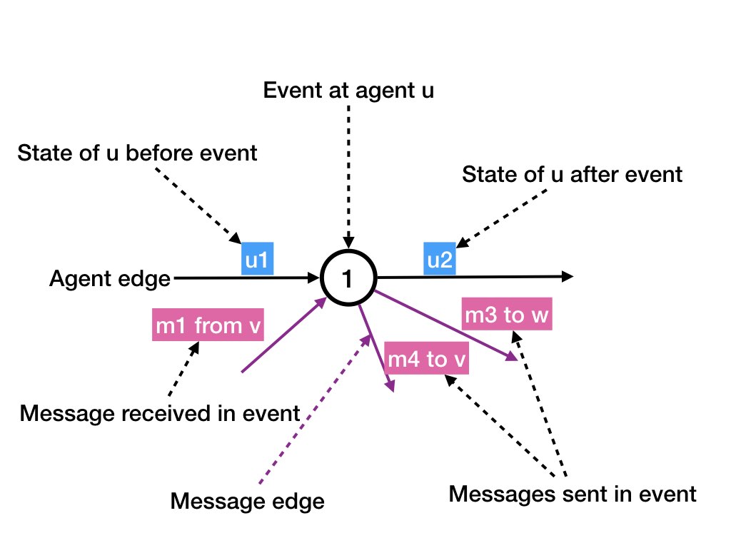
An agent edge is directed from a receive executed by an agent to the next receive executed by the same agent. An agent edge is labeled with the state of the agent between the receives. (This diagram doesn't show labels.)

Steps

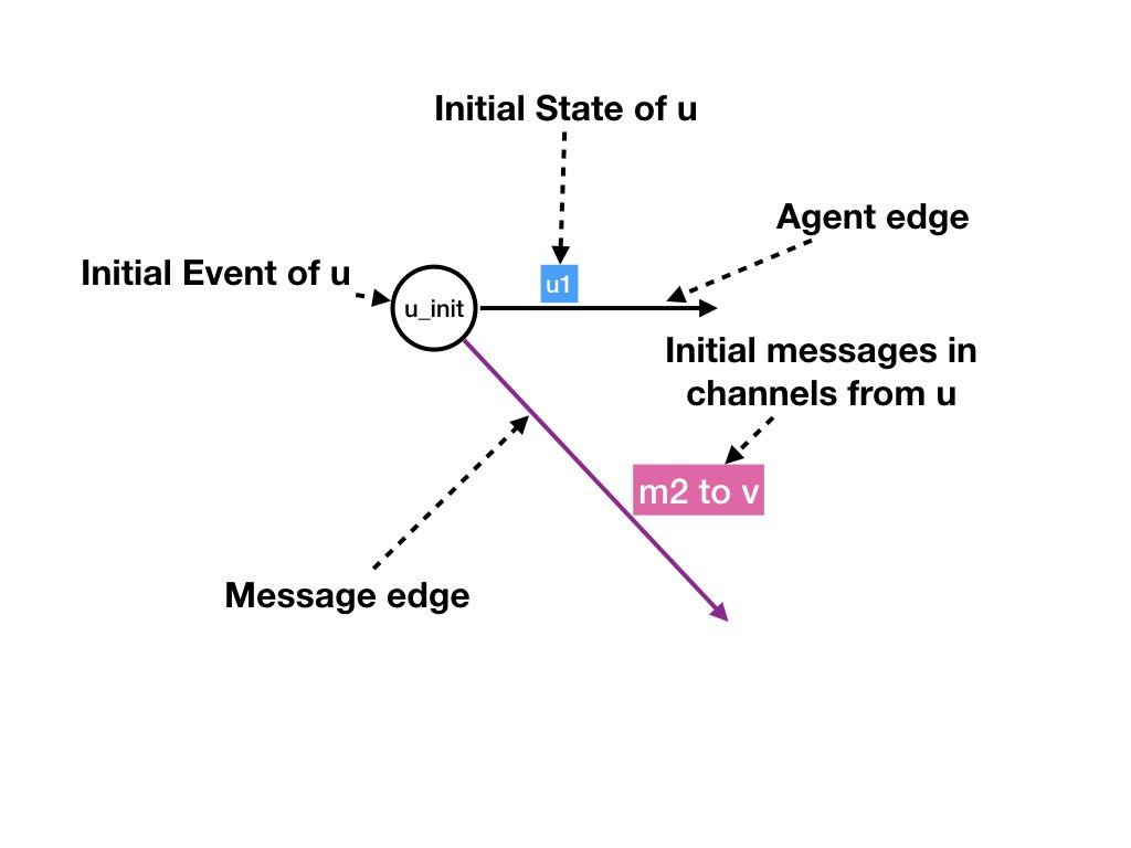
We call the execution of each receive a step in the dataflow graph. Steps and vertices of a dataflow graph are identical. Later we will also use steps in computations.

Fictitious Initial and Final Steps

We have a fictitious initial step for each agent which represents the creation of the initial state of that agent. For example, in figure 4, x_init represents a step that creates the initial state of agent X and also the initial messages in the channels from agent X.

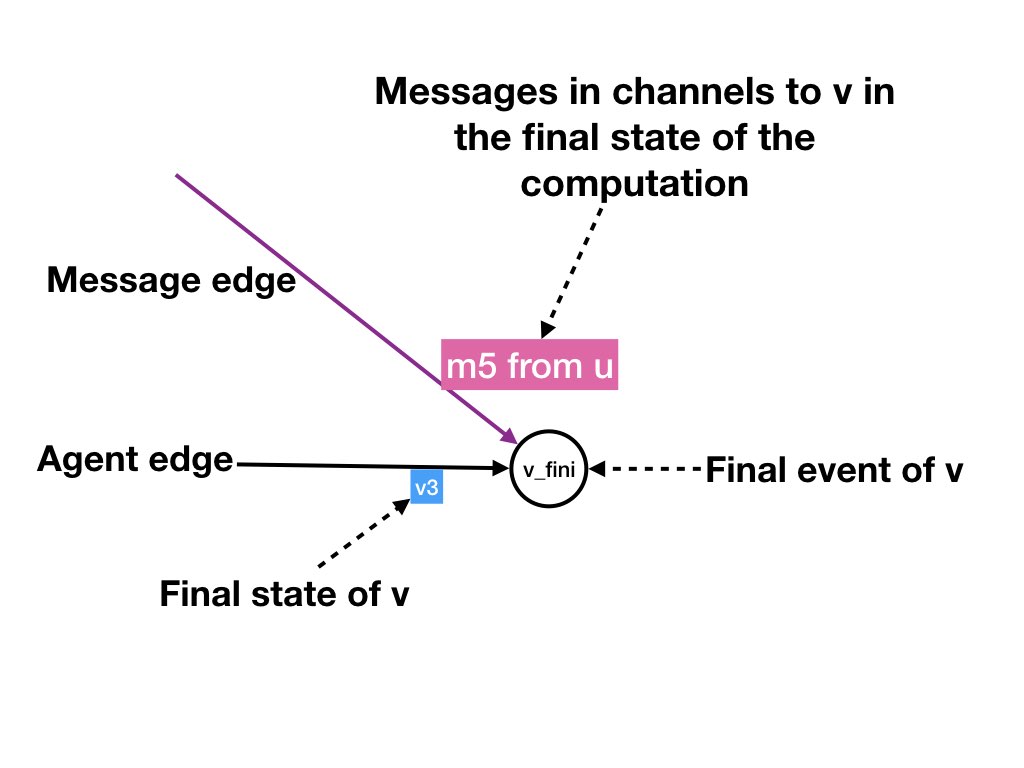
Likewise, we have a fictitious final step for each agent which represents the final state of the agent and the messages in transit to the agent in the final step. For example, in figure 4 there is a message from X to Y, and there is also a message from Z to Y in the final state.

Example of a Dataflow Graph

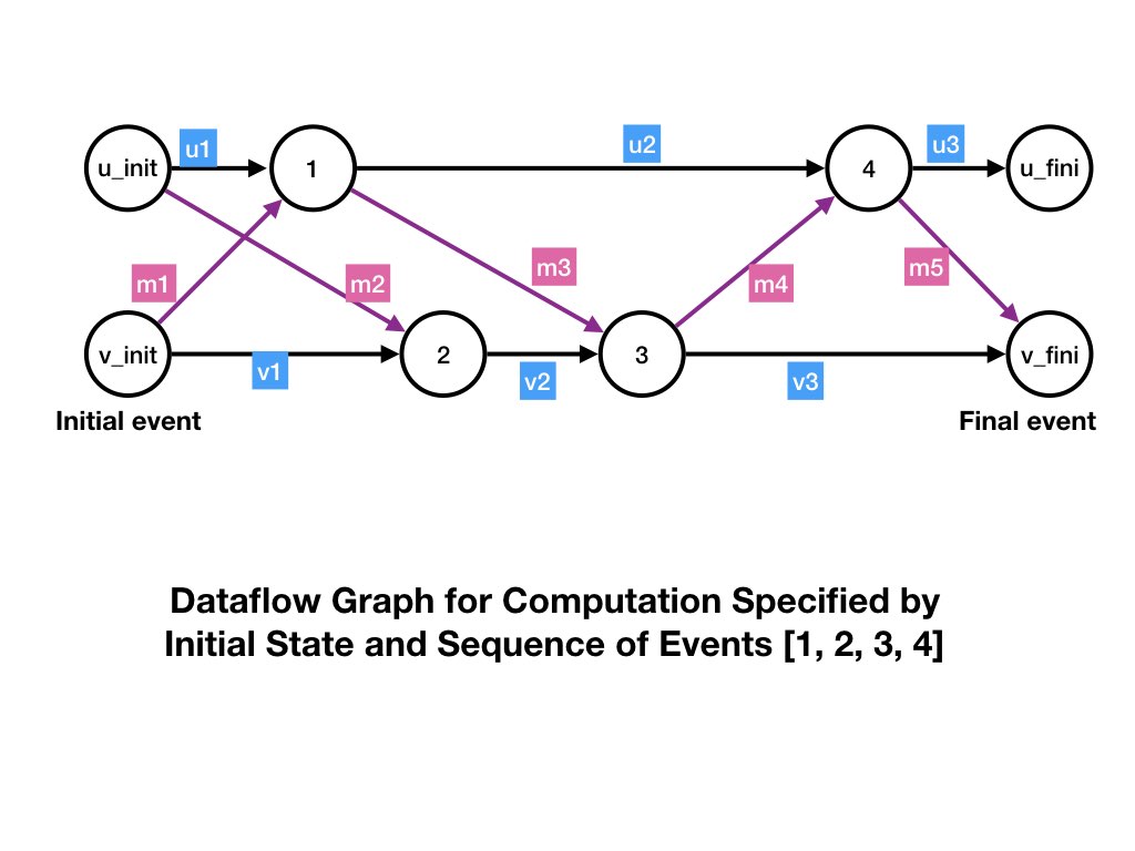
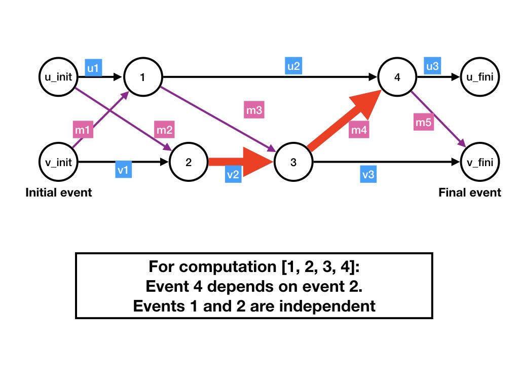
The figure shows the dataflow graph for a system consisting of two agents u and v, and with two channels (u, v) and (v, u). Steps 1 and 4 of the dataflow are at agent u, and steps 2 and 3 are at v. The initial states at agents u and v are represented by outputs of steps u_init and v_init, respectively, and final states by inputs to u_fini and v_fini, respectively.

The labels u1, u2, u3 are: (1) the initial state of agent u, (2) the state of u between steps 1 and 4, and (3) the state of u after step 4, respectively. Likewise, the labels v1, v2, v3 are the states of agent v initially and after steps 2 and 3, respectively.

Message edges are labeled m1, m2, m3, m4, m5. Initially channel (u, v) contains message m2 and channel (v, u) contains message m1. Message m3 is sent in step 1 and received in step 3, and message m4 is sent in step 3 and received in step 4.

Another Example of Timelines and Dataflow Graphs

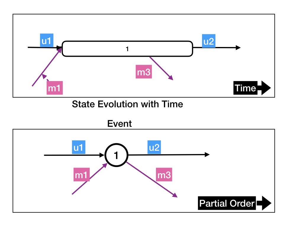
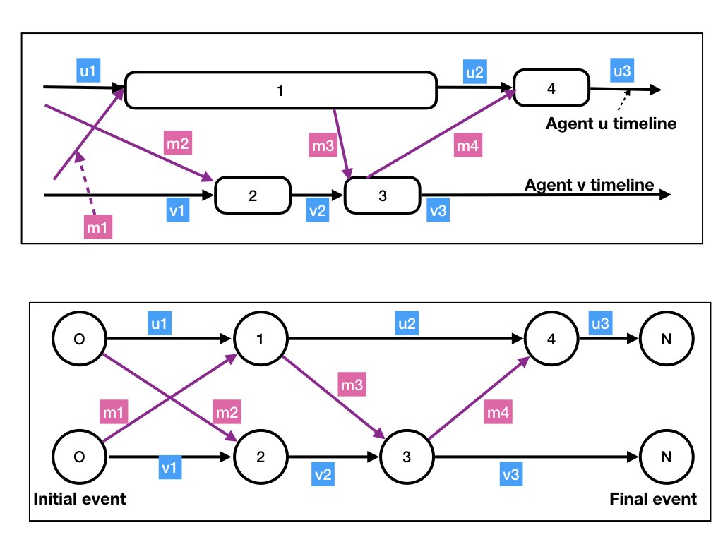
The figure below is an example of a timeline with two agents u and v. Agent u executes two receives represented by rectangles labeled 1 and 4, and agent v executes two receives represented by rectangles labeled 2 and 3. While agent u is executing its first receive (rectangle 1), agent v is also concurrently executing its first receive (rectangle 2). Agent v finishes executing its first receive while agent u is still continuing to execute its first receive. During this execution agent u sends message m3 which is received by agent v which executes its second receive (rectangle 4). Agent v finishes execution of both its receives while agent u is executing its first receive.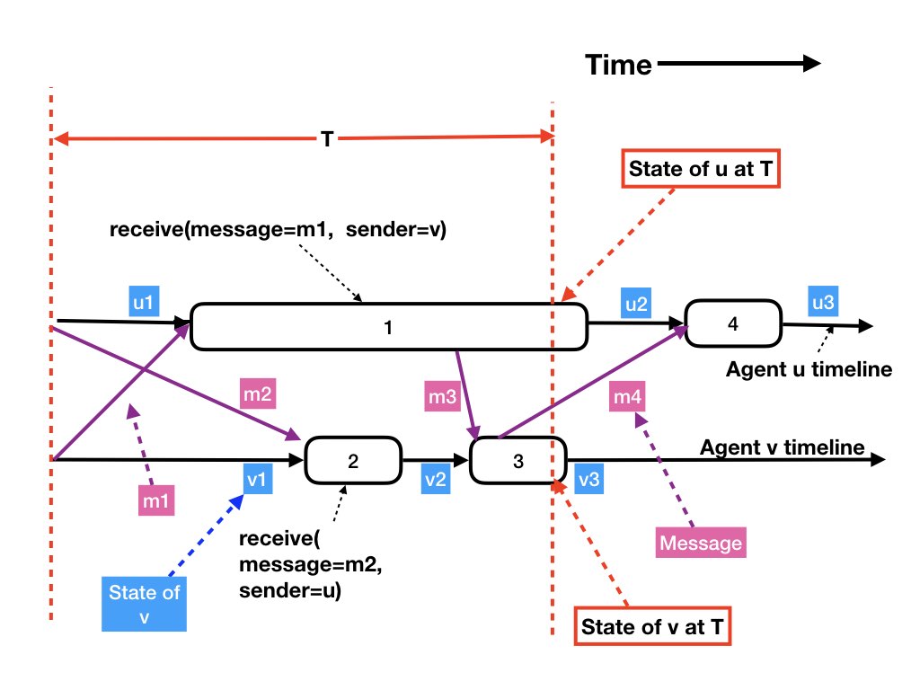

The next diagram shows the abstraction in which an evolution over time is represented by a single event.

The next diagram shows how a timeline is abstracted by a dataflow.

Timelines are important in distributed cyber-physical systems, and we'll look at them later.

Changing the Granularity of States

You may want to analyze system states that include states of an agent while it is executing a receive because analyzing states before and after executing the receive may miss important aspects. For example, suppose the receive function has a while loop and you want to analyze the states of the distributed system after each iteration of the loop. You can make internal states of the receive function observable in the system state by having the agent generate a "next iteration message" from the agent to itself. When the agent receives a "next iteration message" the agent executes the next iteration of the loop. Messages that it receives from other agents are enqueued locally and processed later. So, the granularity of the state space is a design decision.

Flow of Data between Steps

A dataflow graph is acyclic because an edge is directed from execution of a receive function by an agent to a later execution of a receive function by the same agent or the edge is directed from the execution of a receive function in which a message is sent to an execution of a function that receives the message.

The edges of the dataflow graph of a computation show the flow of data into and out of each step. Data -- in the form of the agent's state -- flows from a step at an agent to the next step at that agent. Data -- in the form of message contents -- flows from a step in which a message is sent to the step in which the message is received. We will say that "data flows from a step u to a step v" exactly when there is a path in the dataflow graph from u to v. Some papers use the phrase "u causes v" or "v depends on u." In the figure below, data flows from step 2 to step 4, or equivalently step 4 depends on step 2.

We say that two vertices (steps) of a dataflow graph are independent exactly when there is no path between the vertices.

Agent logs specify a unique dataflow graph but not the ordering among independent steps

Given the logs that agents make during an execution of a system, there is a unique dataflow graph that is consistent with the logs. The logs specify a unique dataflow graph but do not specify the order of execution of independent events. For example, the logs in the figure below do not specify whether step 1 occurred before, after or during step 2.

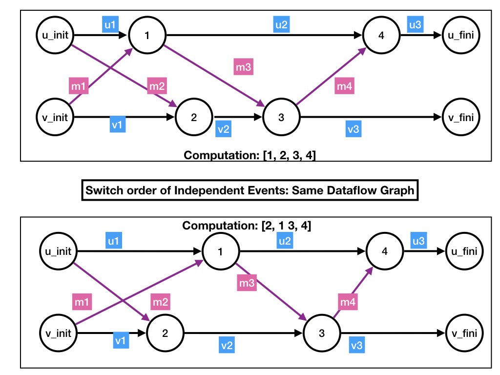
The diagram on the top illustrates a sequence of steps 1, 2, 3, 4 while the lower diagram illustrates sequence 2, 1, 3, 4. Both diagrams have the same agent logs, and therefore the same dataflow graph.

States

The future behavior of a system from its current state is independent of the system's past behavior.

The state of a distributed system is given by the states of its agents and channels. A system state is a tuple with an element of the tuple for the state of each agent and each channel. The state of a channel is a queue consisting of the sequence of messages sent on the channel that have not been delivered. The state of an agent is given by the values of its variables.

See examples of states and state transitions and questions about states of distributed systems.

State Transitions and Events

There exists a transition from a state S to a state S' exactly when in state S there is a nonempty channel (v, u) and the delivery of the message m at the head of the channel to agent u and the execution of receive(message=m, sender=v) by agent u causes a transition to state S'. The change in state is specified by the 4-tuple:

1. u's state s before it executes the receive.
2. The sender, v, of the message, and the message, msg, that is received,
3. u's state s' after it completes execution of the receive.
4. For each channel (u, v) from u, the sequence of messages that u sends along the channel while it executes the receive. The sequence of messages is the empty sequence if u sends no messages along the channel during the receive.

The 4-tuple is called an event. The first two elements of the tuple are called the inputs to the event, and the last two elements are the outputs of the event. The states of all agents other than u remain unchanged in this transition. The states of channels not listed in the event also remain unchanged. The only changes in a state transition are changes to a single agent and the channels incident on that agent.

Each vertex of the dataflow graph represents the execution of an event.

The same event can occur multiple times in a dataflow graph. This is because an agent may execute a receive function with the same input and in the same state multiple times. So, there may be multiple vertices of the dataflow graph with identical labels of inputs and outputs. Each execution of a receive function is a different step of the dataflow graph. So, there may be multiple vertices with identical inputs and outputs, and each of these vertices is a different step.

We assume that the receive function is deterministic. The output of an event is a function of its input.

If all channels are empty in a state S then there is no transition from S.

Locality of Events

An event specifies the state transition of a single agent and the edges incident on it when the agent executes its receive function; the event does not specify the states of other agents and channels. A transition from a state S to a state S' specifies the states of all agents and all channels in S and in S'. A state transition specifies the global (entire) state of a system before and after the transition. In contrast, an event specifies the local states of a single agent and its incident edges before and after the transition.

Example of State Transitions and Events

This example is of an event at agent, pos from the previous page. In this example,the state of pos before the event is given by the values of its variables my_data = [3, 5] and n = 0. In the event, pos receives a "wakeup" message from itself. A wakeup message is shown as a star in the diagram.

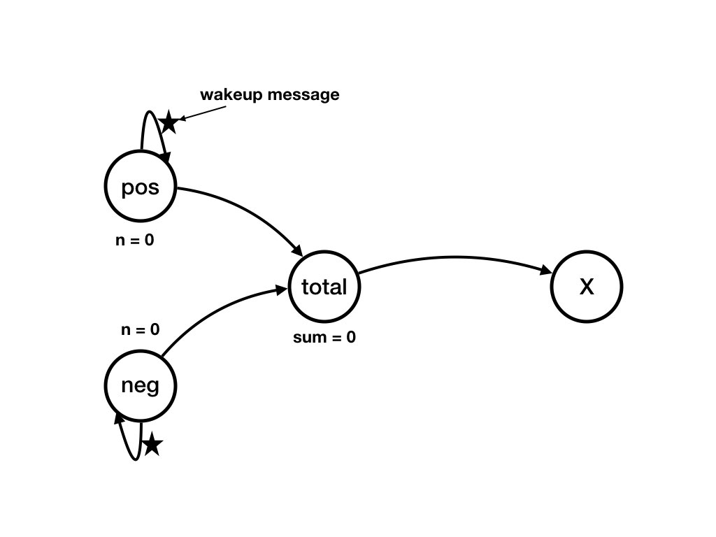
The execution of the event (receive('wakeup', pos)) causes a state transition from state S_0, shown in the figure above, to state S_1, shown in the figure below.

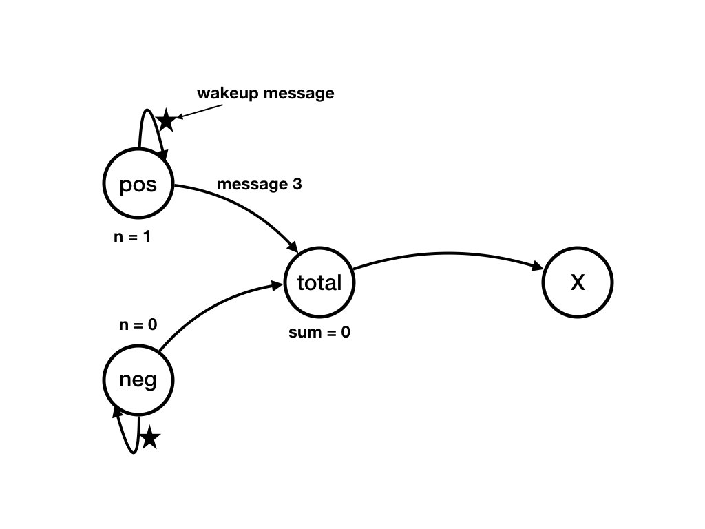
pos's state after the event is my_data = [3, 5] and n = 1. During the event pos sends a "wakeup" message to itself and sends 3 to agent total. The event is specified by the following tuple:

1. pos's state before it executes the receive is given by the values of its variables my_data = [3, 5] and n = 0.
2. The sender of the message that is received in this event is pos, and the message is "wakeup".
3. pos's state after it completes execution of the receive is given by my_data = [3, 5] and n = 1.
4. The messages sent during the execution of receive are (i) "wakeup" to pos and (ii) 3 to total.

The states of the other agents -- neg, total, and X -- remain unchanged in this state transition. Likewise, the states of channels that are not incident on pos -- channels (neg, neg), (neg, total), and (total, x) -- remain unchanged in the transition.

Computations

A computation is a sequence of states, where there exists a transition from each state in the sequence to the next. A computation may be finite or infinite. A computation may start in any state. We will often prove properties of computations that start in an initial state of the system; however, a computation is not restricted to starting in an initial system state.

Example of a Computation

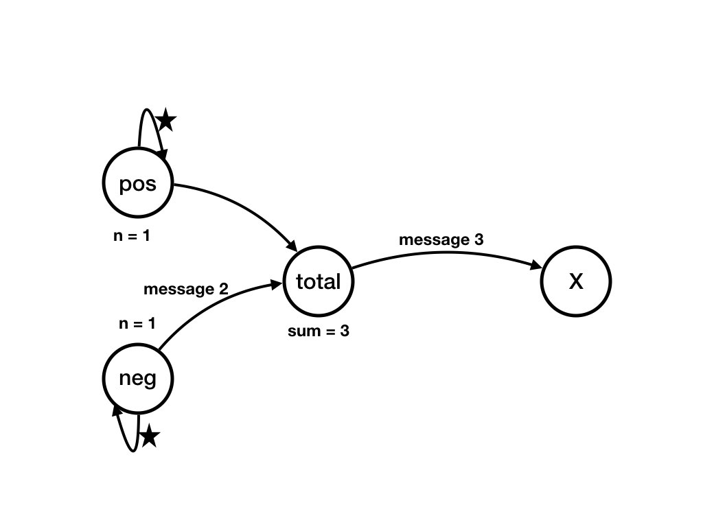
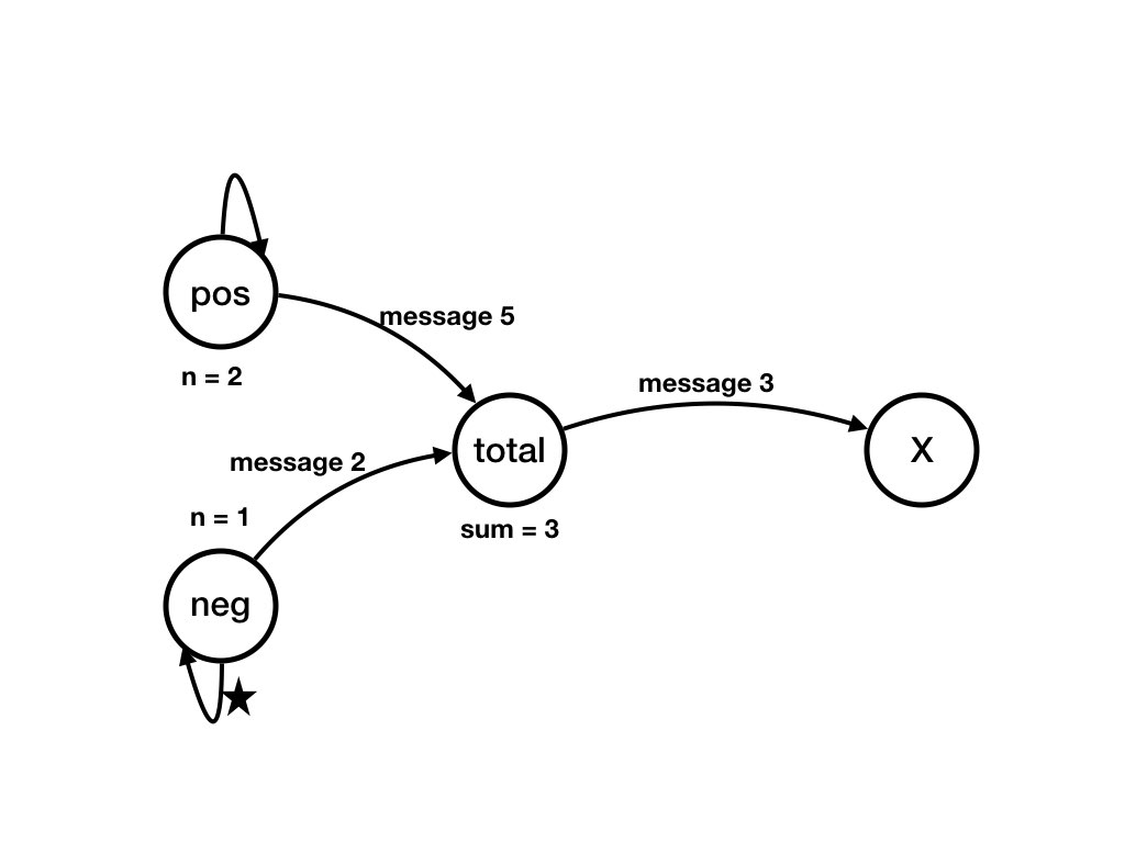
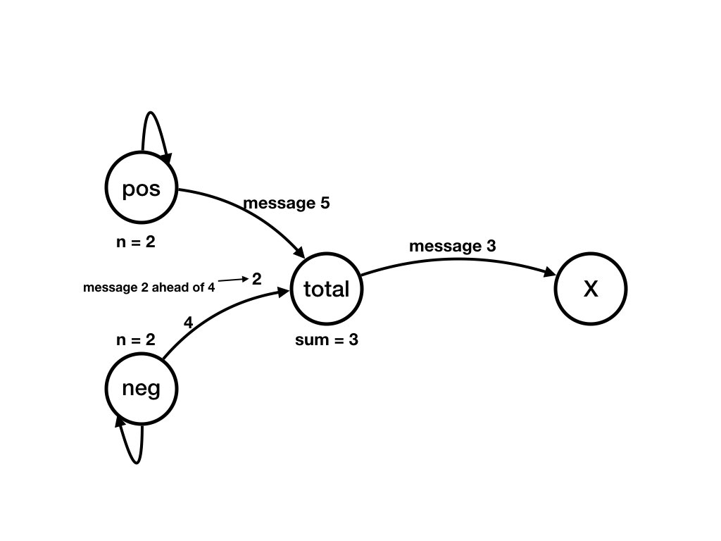
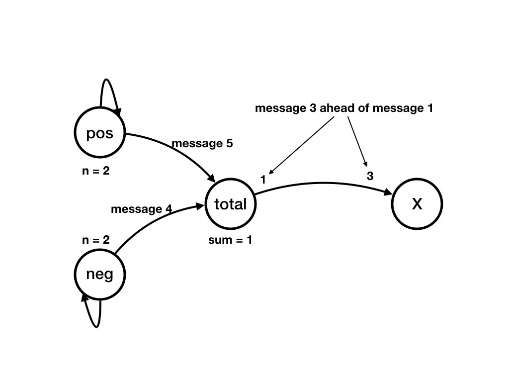
The next series of figures shows a computation. Each figure shows a state. There is a transition from the state shown in a figure to the state shown in the next figure. There is a computation that starts in the state shown in the first figure below to the state shown in the last figure.

Every subsequence of a computation is also a computation. For example, there is a computation that starts in the state shown in the second figure to the state shown in the fifth figure.

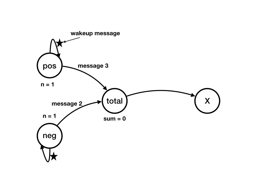
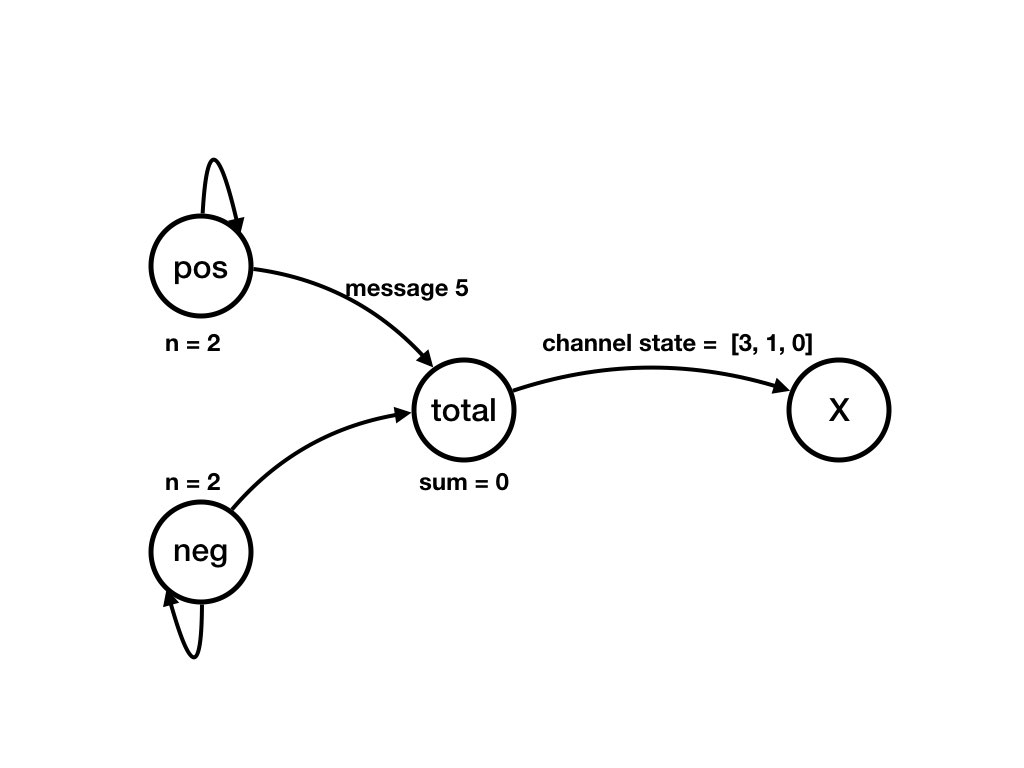
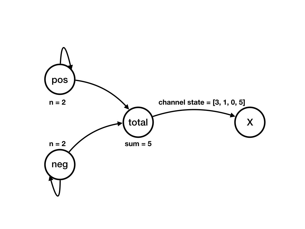
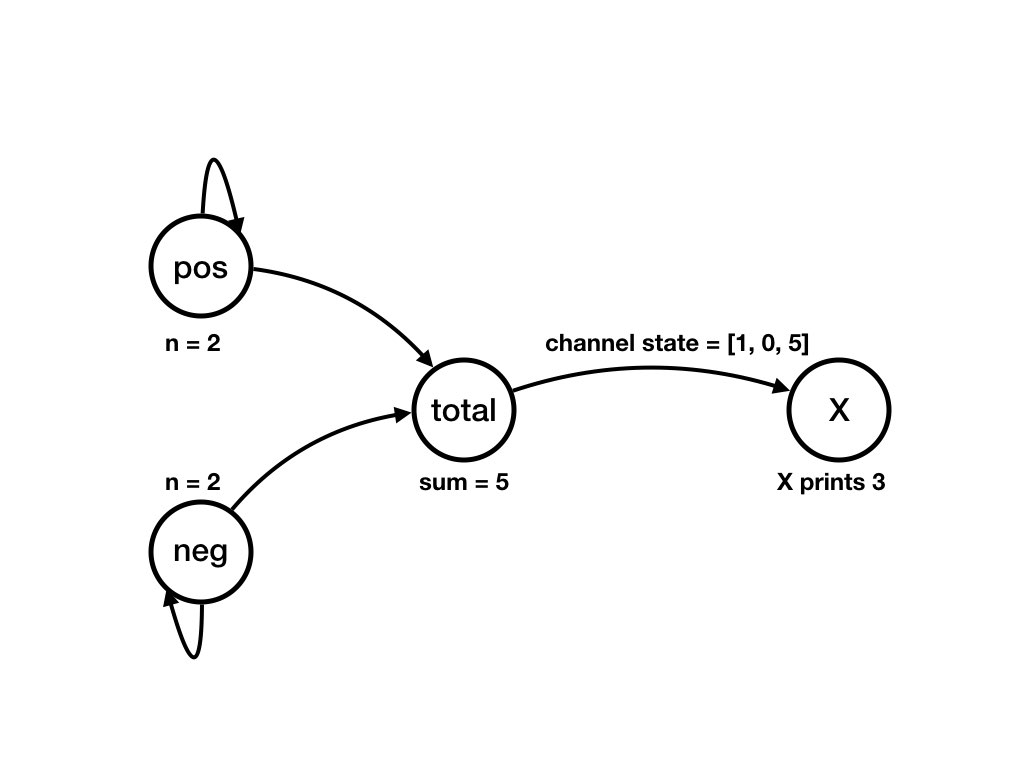
Sequential Program Representation of Computations

All computations starting from a state \(S_{0}\) are sequences \([S_{0}, S_{1}, S_{2}, \ldots, ]\) of states generated in the following while loop.

---

# The initial state is S[0]
step_number = 0
while there exists a nonempty channel:
   # state is S[step_number]
   select any nonempty channel (v, u)
   let m be the message at the head of (v, u)
   deliver m to agent u which executes receive(m, v)
   step_number = step_number + 1

---

The loop terminates when all channels are empty. The selection of the nonempty channel in an iteration is nondeterministic -- any nonempty channel can be selected. Different computations are generated by making different selections of the nonempty channel in each iteration. When we prove properties of computations we have to consider all possible selections of nonempty channels.

A benefit of using the states in a while loop to represent the states of a computation is that we can use familiar techniques --- such as loop invariant and loop variants --- for reasoning about sequential programs to reason about distributed algorithms as well.

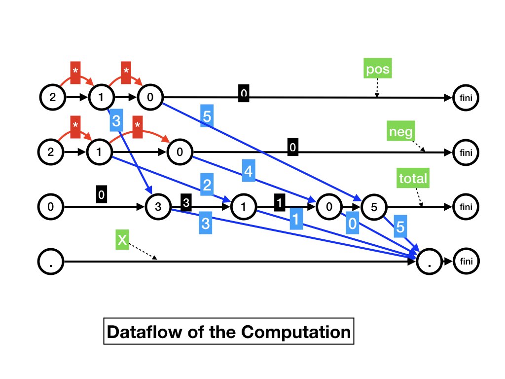
Dataflow Graph of a Computation

Each computation has a unique dataflow graph associated with it. The steps of the dataflow graph are executions of receive functions in the computations. The agent and message edges of the dataflow graph of the computation are as given before.

A computation is a total ordering of executions of receive functions. A dataflow graph is a partial ordering of executions of receive functions because the graph is acyclic. Many computations can have the same dataflow graph.

The figure above shows the dataflow graph for the computation shown in the previous diagrams. The black edges are agent edges and they are labeled with the states of agents. The blue and red edges are message edges and are labeled with the contents of messages. The red edges show internal messages, i.e., messages from an agent to itself. The top row shows steps at agent pos, the next row shows steps at agent neg, and the bottom two rows shows steps at agents total and X. The numbers inside the steps for pos and neg are the value of n at steps. The numbers inside the steps for total show the value of sum. Not all labels on agent edges are shown in the diagram.

Topological Sorts of Directed Acyclic Graphs

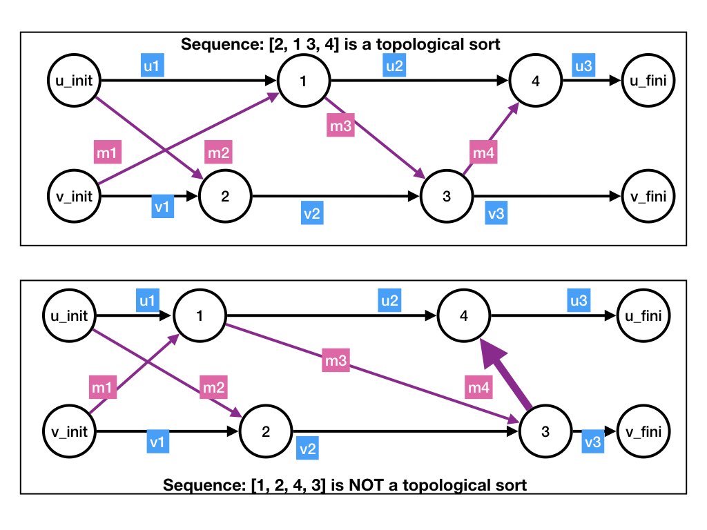
A topological sort of a directed acyclic graph is a sequence of vertices of the graph where for every edge \((x, y)\) in the graph, \(x\) appears before \(y\) in the sequence.

Examples of Sequences that Are and Are Not Topological Sorts

Sequences [1, 2, 3, 4] and [2, 1, 3, 4] are topological sorts of the graph. Sequence [1, 2, 4, 3] is not a topological sort because there is a backward edge , i.e., an edge directed from a later vertex in the sequence (i.e, vertex 3) to an earlier vertex (4) in the sequence.

---

Theorem: Topological Sorts of Dataflow

All topological sorts of a dataflow graph of a computation are computations.

---

Proof of the Theorem

Let \(G\) be the dataflow graph of a computation specified by a sequence of steps \(E = [e_{0}, e_{1}, \ldots]\). Let \(E'\) be a topological sort of \(G\). We will prove that \(E'\) is also a computation.

The theorem holds trivially if \(E'\) and \(E\) are identical. If \(E\) and \(E'\) are not identical then there exists an adjacent pair of steps \(e_{i}, e_{i+1}\) in \(E\) where \(e_{i+1}\) occurs before \(e_{i}\) in \(E'\). Because \(E'\) is a topological sort, there is no edge in the dataflow graph from \(e_{i}\) to \(e_{i+1}\).

Let \(H\) be the sequence of steps identical to \(E\) except that the order of \(e_{i}\) and \(e_{i+1}\) is switched in \(H\). From the lemma \(H\) is also a computation. The number of out of order pairs between \(H\) and \(E'\) is less than that between \(E\) and \(E'\). By repeatedly switching independent, adjacent, out-of-order pairs the sequence \(E'\) is reached.

Equivalent Statements of the Theorem

---

A sequence of steps of a dataflow graph is a computation exactly when: For all steps v, w in the graph where there is a path from v to w: v appears before w in the sequence.

---

Equivalently, a sequence of steps is a computation if for all steps v, w: if data flows from v to w then v appears before w in the sequence.

We may also use phrases such as "data flows forwards" in a computation or "each step depends only on earlier steps" of a computation.

Model Strengths and Limitations Limitations

Agents in many distributed systems have semi-synchronized clocks; though the clocks are not perfect, they do not drift apart by arbitrary amounts. The time that a message is in flight in some distributed systems can be bounded. Distributed cyber-physical systems have clocks that are synchronized (if imperfectly) and assume bounds on message delay. The model that we have described is inappropriate for such systems. Later we discuss models that do include clocks and bounded message delays.

A dataflow graph faithfully represents the flow of data between steps; however, a dataflow graph is not a timeline. Dataflow is adequate for many distributed applications.

A state transition represents a change from a state in which all agents are idle to a state in which all agents are idle. The transition captures the change in state of exactly one agent when it executes a receive. A computation is a sequence of states where all agents are idle in every state in the sequence. Restricting consideration of states in which all agents are idle may seem a severe limitation of the model.

As we saw, the sequence of states of a computation are the states in a sequential nondeterministic while loop. It may appear that the model is weak because we are representing dynamic, multi-agent, concurrent systems by sequences. We will see that these limitations are not restrictive.

Next

The next pages describes Cuts in Dataflow Graphs which are used in developing detection algorithms such as termination detection and deadlock detection.

Examples

Frequenty Asked Questions

Review

---

K. Mani Chandy, Emeritus Simon Ramo Professor, California Institute of Technology